|
Raspberry Pi based Digital Measurement System in Physics
|
||||||
|
||||||
|
|
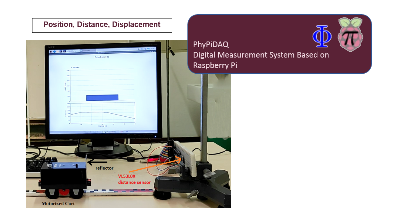
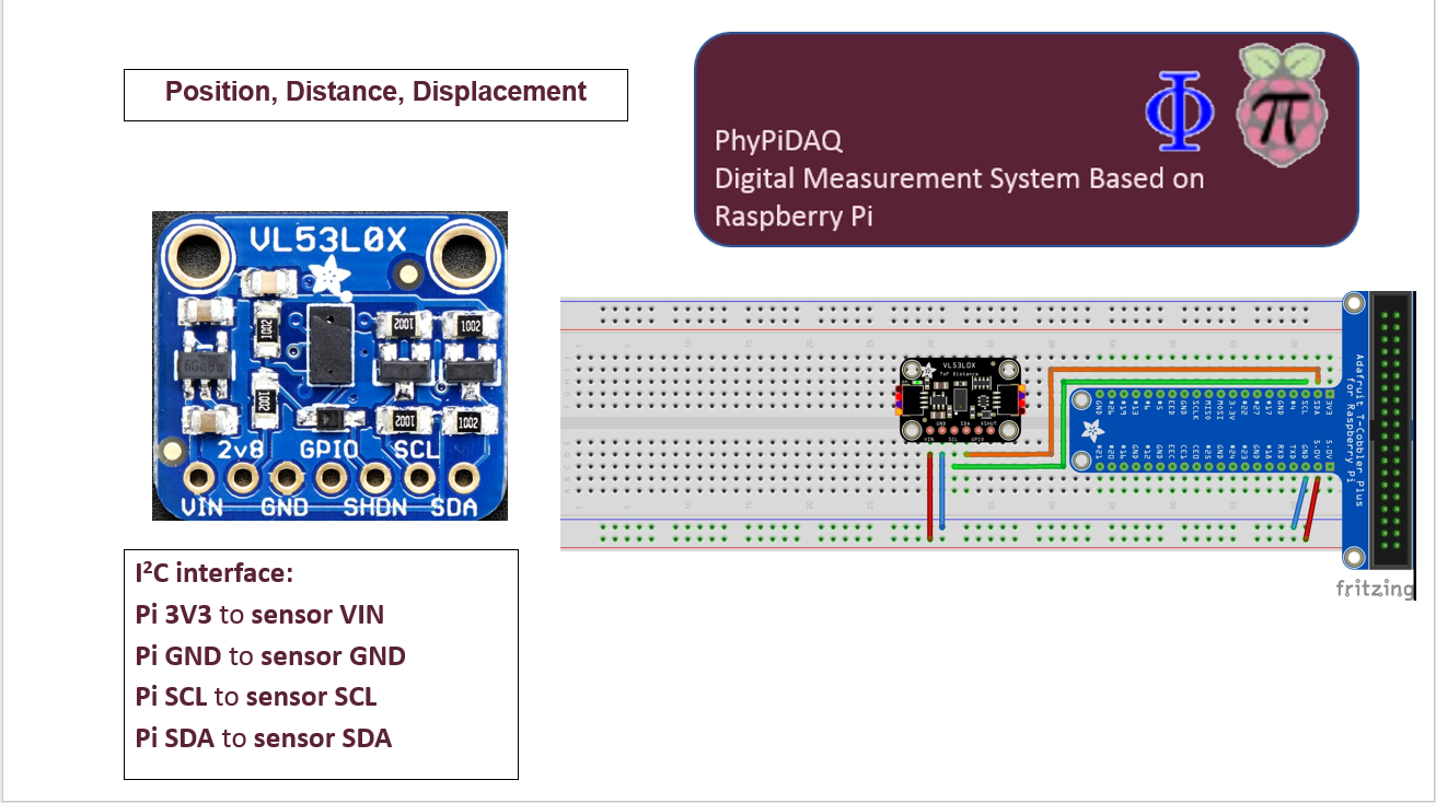
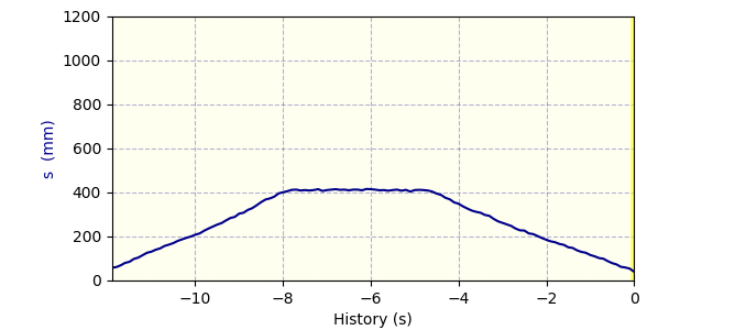
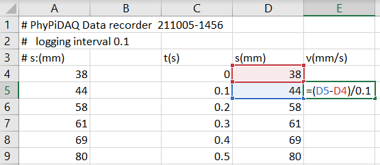
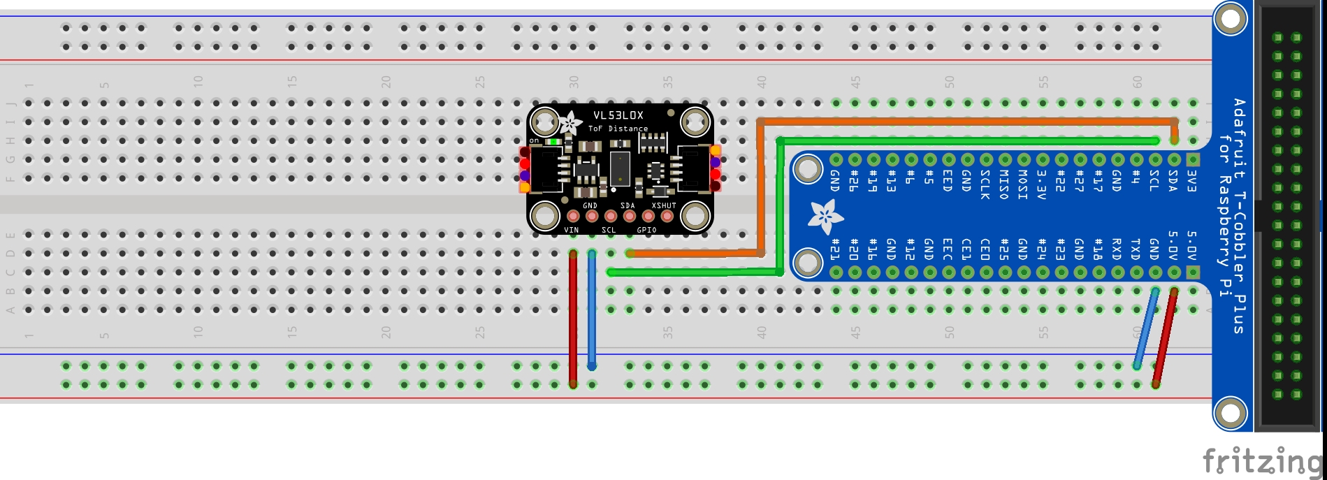
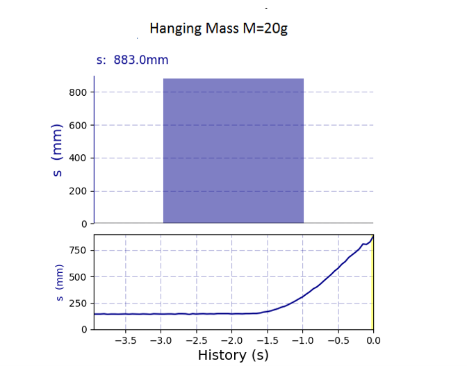
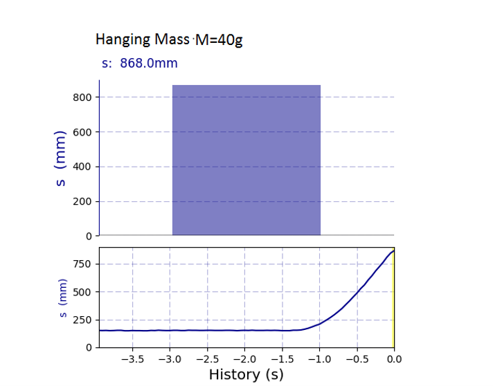
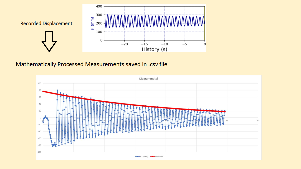
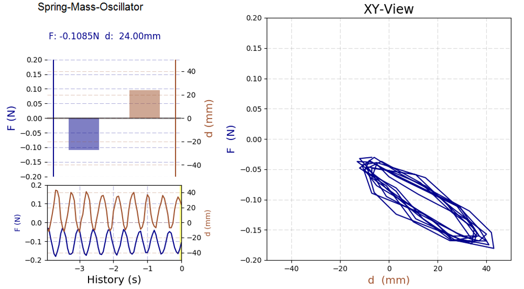
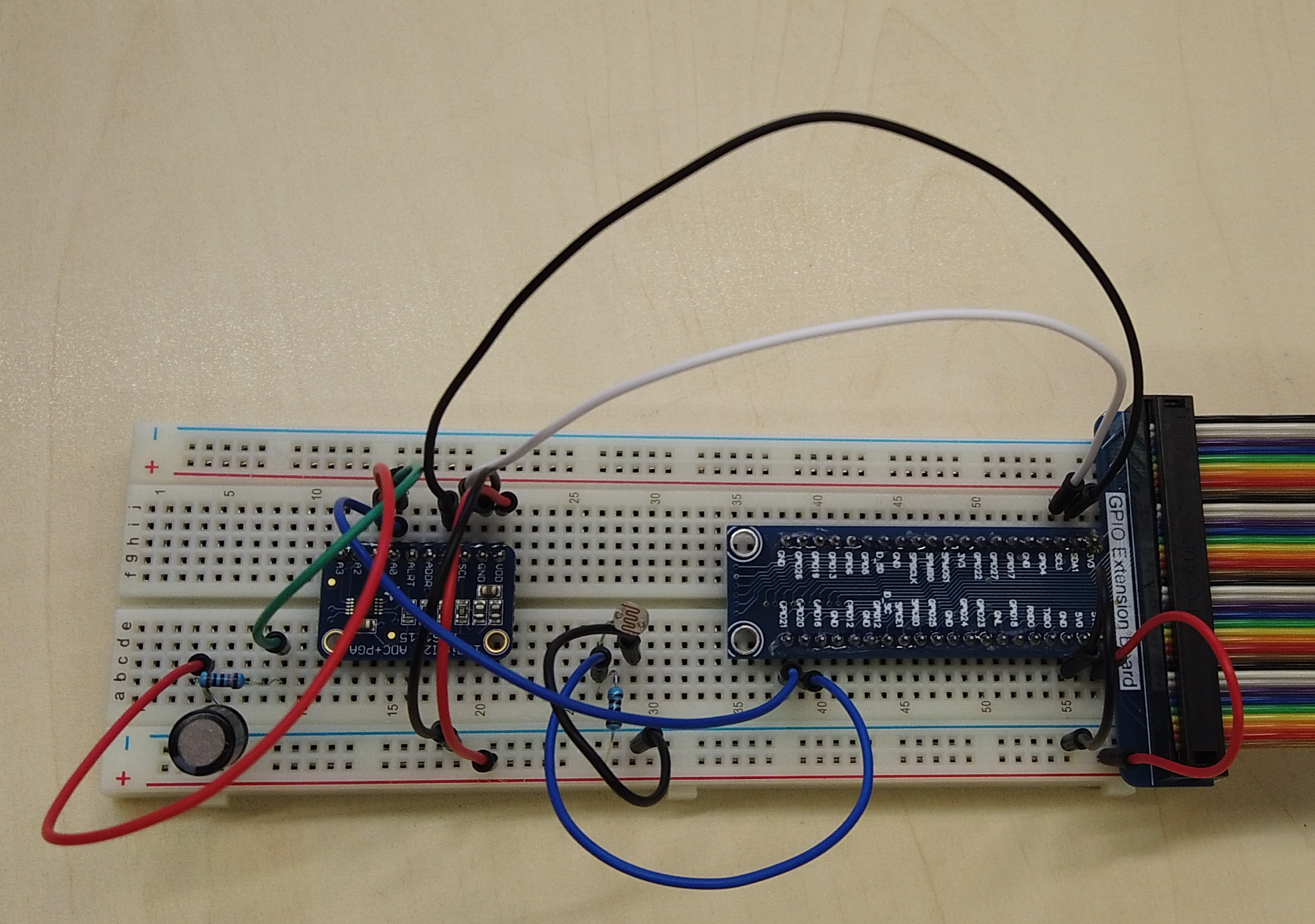
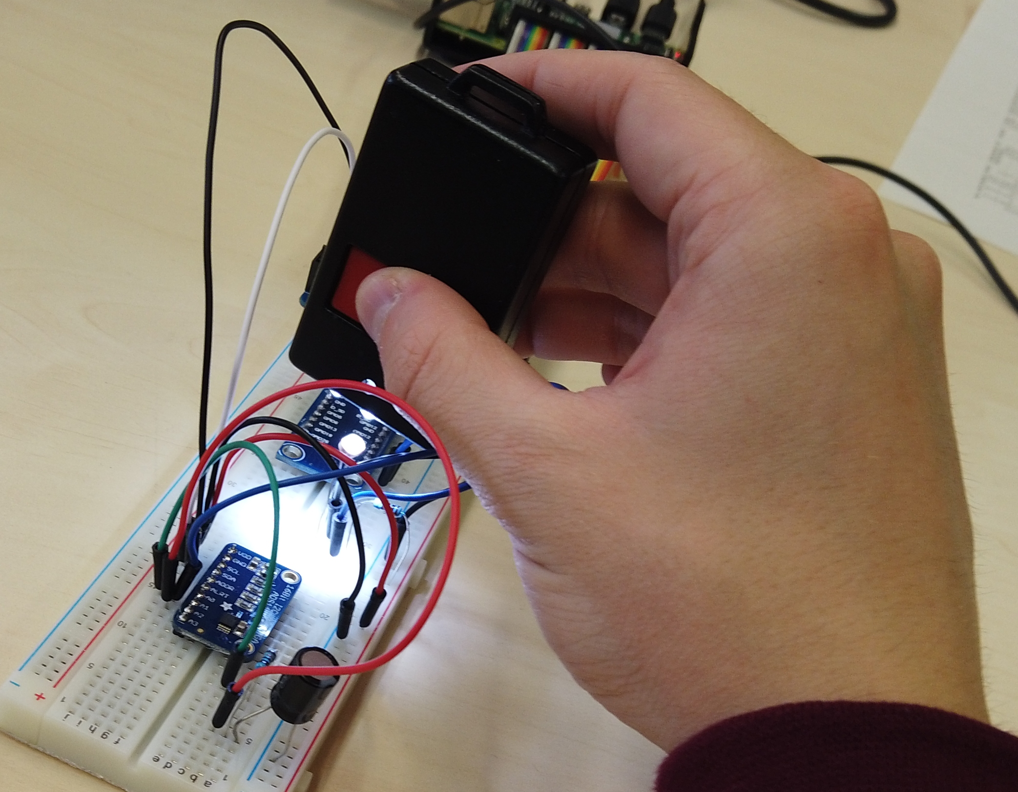
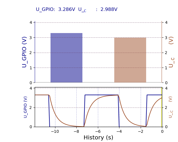
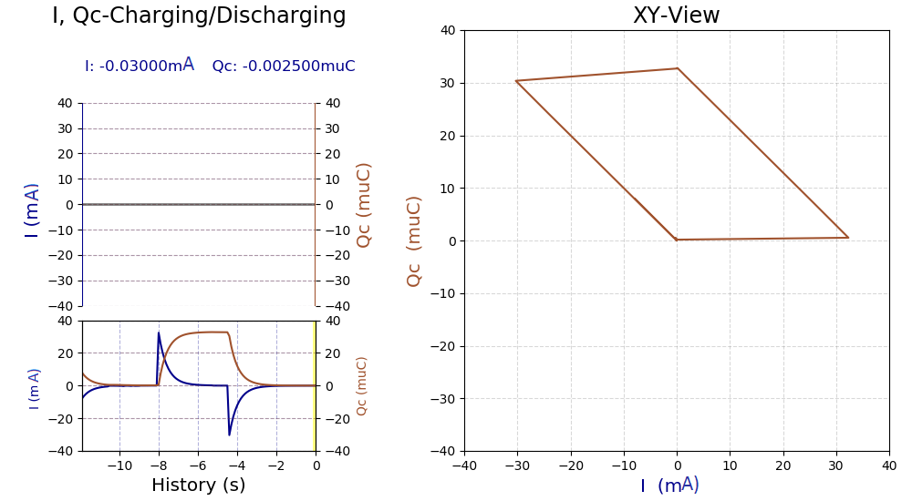
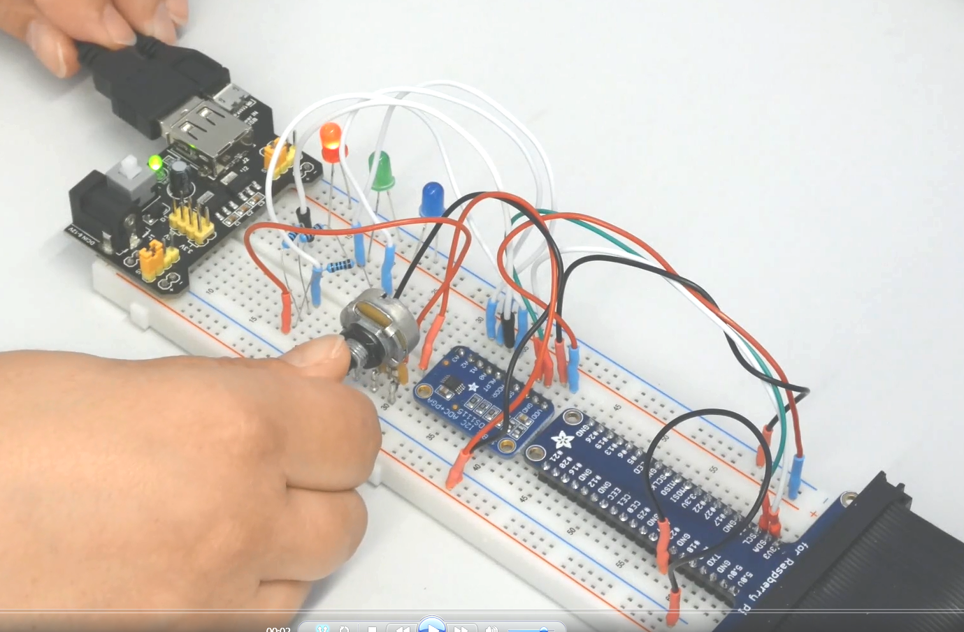
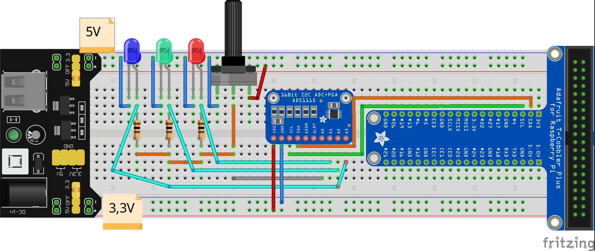
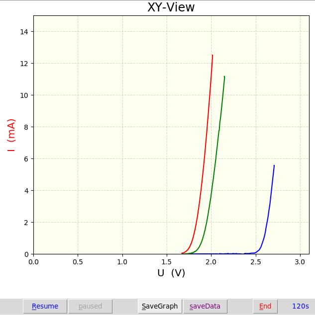
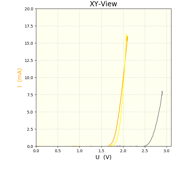
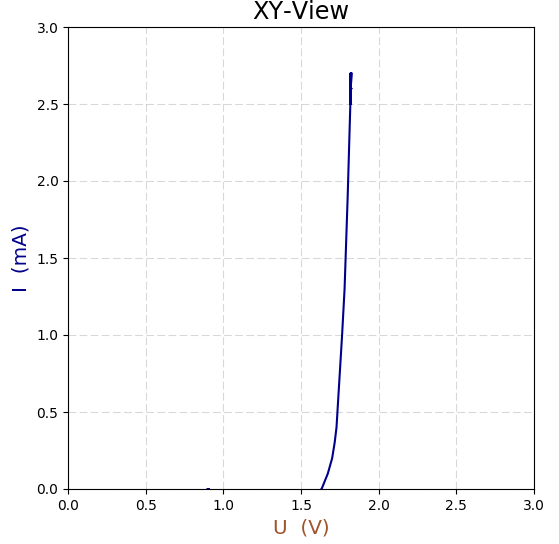
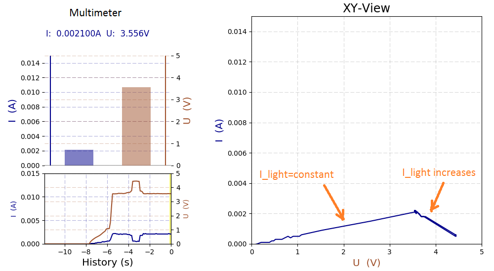
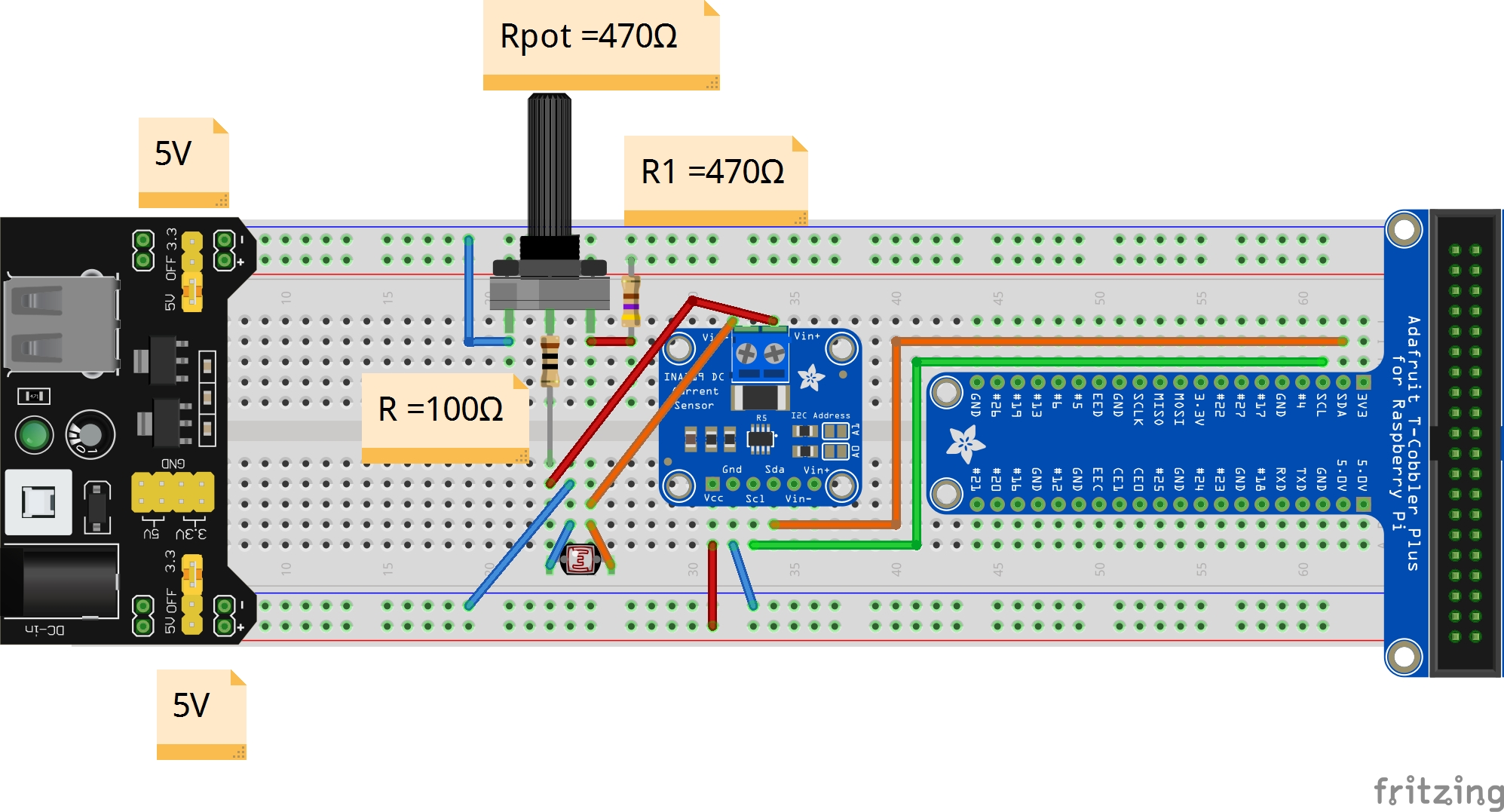
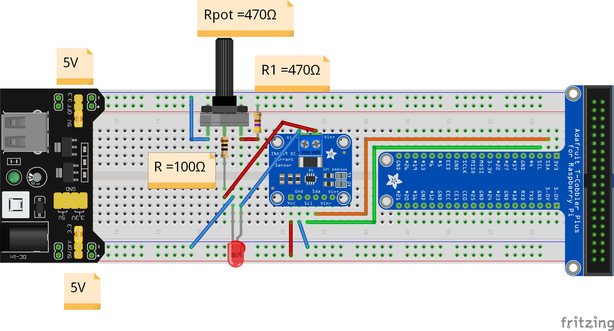
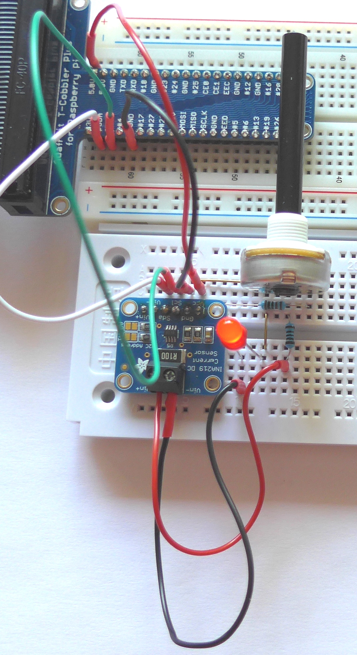
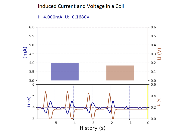
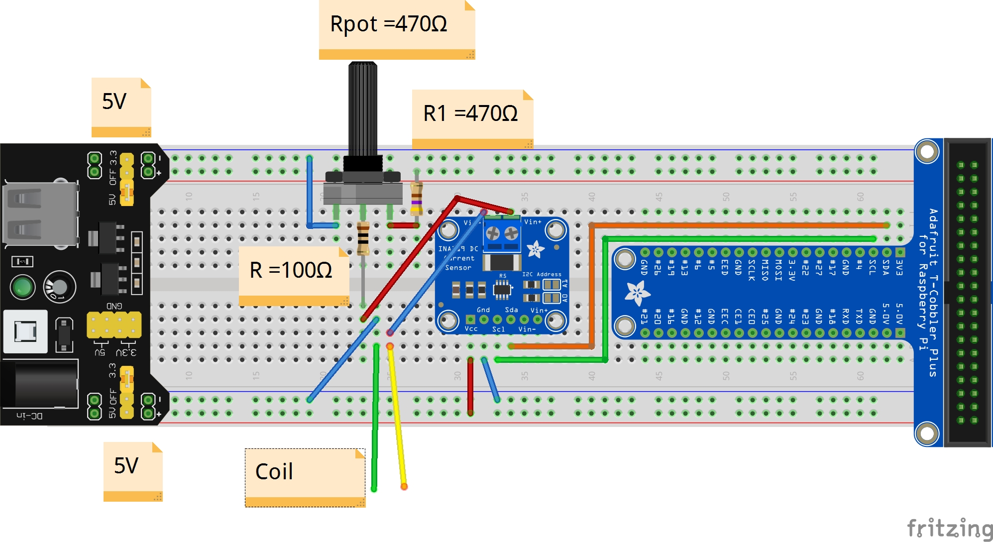
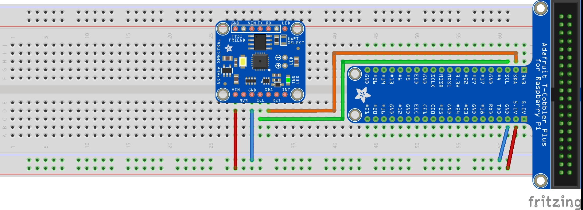
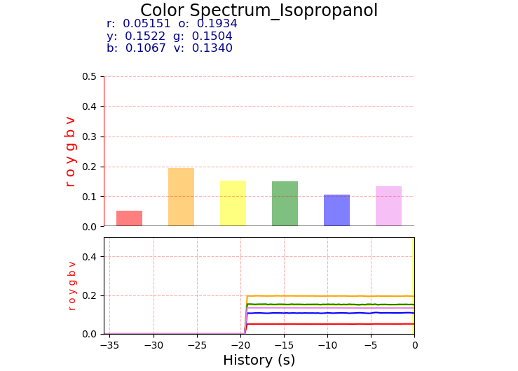
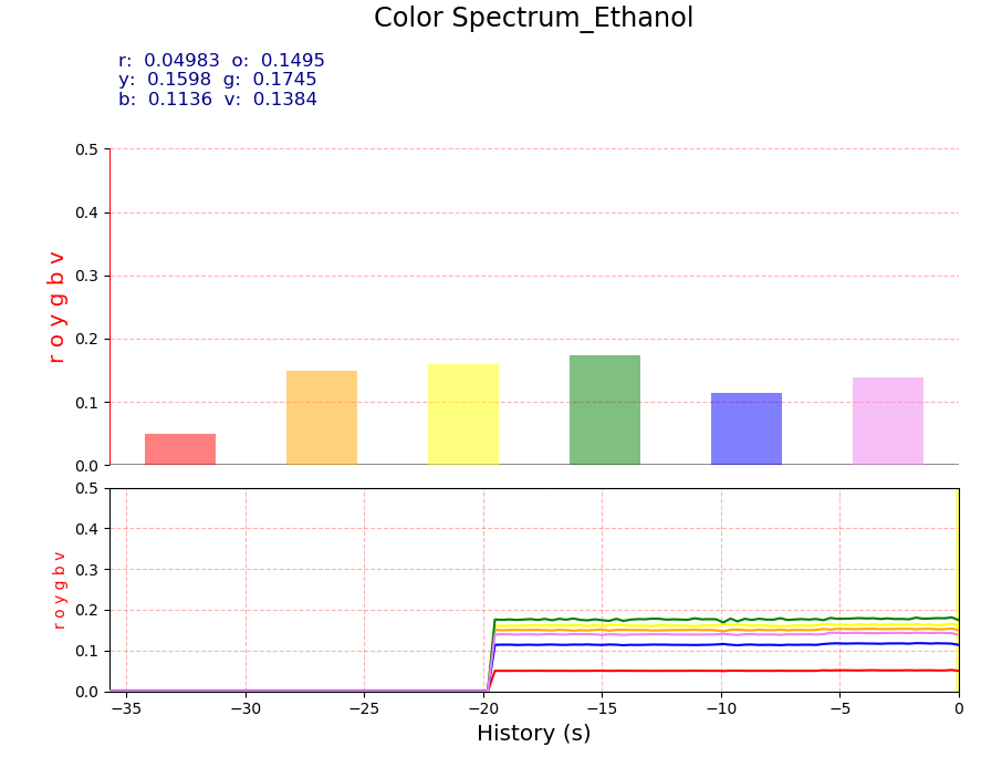
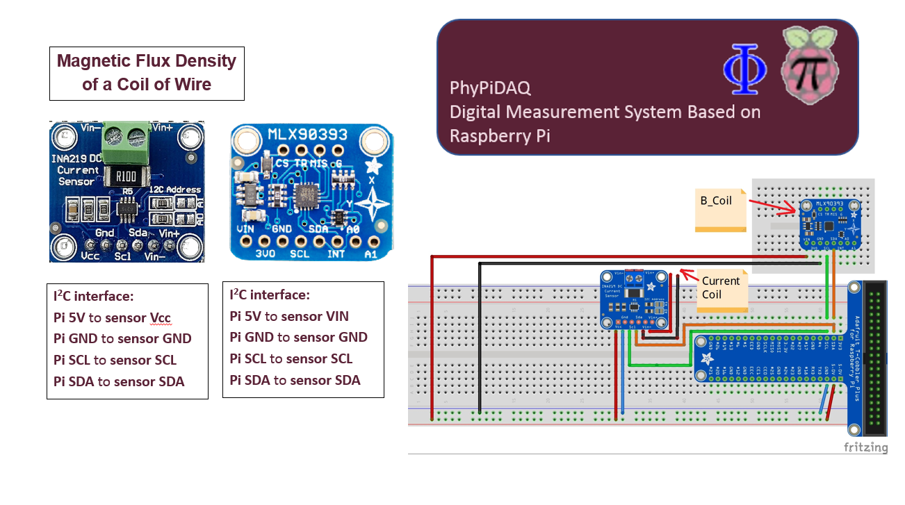
The Activity-Based Physics contains folders consisting of pre-configured modules of specific sensors such as sensors for position, acceleration, temperature, current, etc. having the extension .yaml. Moreover there are modules with built-in commands of type .daq to configure the experiments. These configurations assigned to specific experiments are saved in .pdf format. In the /home/pi/git/PhyPiDAQ/examples folder, which has been installed together with the PhyPiDAQ-Software, one can choose the available .daq configuration for the desired experiment, and then change the instructions according to the recommended commands which are highlighted in the .daq and .yaml configuration saved in .pdf format. As another option, one can choose the default.daq configuration, also available in the /home/pi/git/PhyPiDAQ/examples folder. This configuration is convenient for all sensors and can be customized for different experiments by introducing channel limits, physical quantities, units of measurements, different display modules, and saving of measured data capability. In the configuration of each sensor or measuring device saved under SensornameConfig.yaml there are features like measuring ranges, number and type of channels, values limits, that students select in the graphics window of the interface according to the experimental purposes. Additionally, each Activity-Based Physics folder contains pictures of the circuit showing how to connect different sensors to the Raspberry Pi. In each Activity-Based Physics folder, there is a file of type .daq to configure the graphical display of the measurements. Built-in commands and instructions allow the user to pick different display modes, like the graph of measured quantities over time by choosing DisplayModule: DataLogger, instant bar charts of measured signals to quickly compare data and, to highlight specific values at a glance by choosing DisplayModule: DataGraphs, or XY-graphical relationship of physical quantities if using multiple sensors at the same time. Some sensors, such as INA219, record physical quantities on more channels so that their relationship can be visualised by way of XY-graphical representation. Other data visualization capabilities, like introducing title, measurement name and units, proper graphical ranges, as well as the conversion of the output sensors' voltage into physical quantities or use of formulae for displaying desired quantities are provided. The PhyPiDAQ software gives also the possibility to store the measured data, which can easily be converted to a format compatible with spreadsheets such as Excel or LibreOffice running directly on the Raspberry Pi for more extensive analysis. The .csv files in the Activity-Based-Physics folders are assigned to each experiment and hold recorded data from previously run experiments. These data can be further processed by way of employing spreadsheets such as Excel or LibreOffice. They are very suitable for physical and mathematical applications regardless of whether the experiment has been run before.
|